Features

There are two kinds of features unique to time series

• time-step features
  • e.g. time dummy, which counts off time steps in the series from beginning to end.
• lag features
  • e.g. n-step lag

Common Patterns

• trend (deterministic features)
• seasonality (deterministic features)
  • can be visualized with Periodogram
• autocorrelation = the correlation a time series has with one of its lags
• noise
• non-stationary: the data will vary in accuracy at different time points

Components

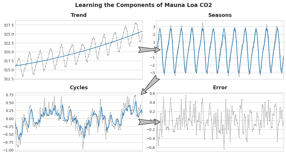
• Many time series can be closely described by an additive model of just three components, trend, seasons, and cycles, plus some essentially unpredictable, entirely random error:

series = trend + seasons + cycles + error

``

Forecasting

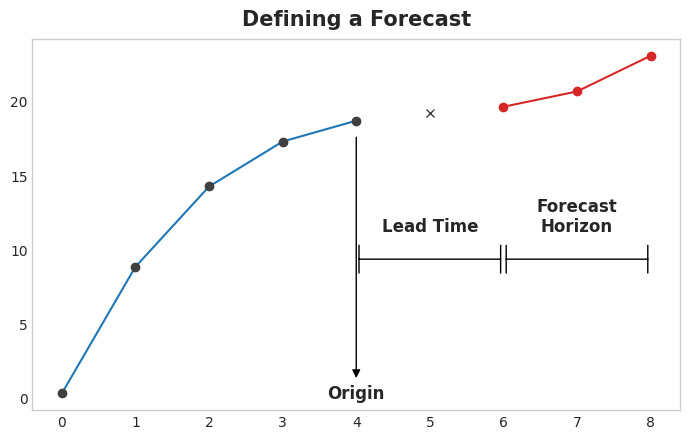
Defining the Forecasting Task

• There are two things to establish before designing a forecasting model:
  • what information is available at the time a forecast is made (features)
  • the time period during which you require forecasted values (target)
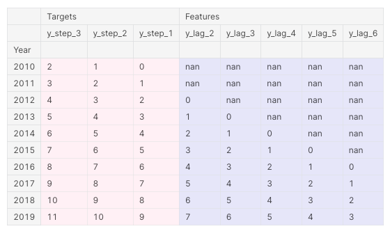
• example: a three-step forecasting task with a two-step lead time using five lag features
  
  corresponding preprocessed dataframe
  

Common Multistep Forecasting Strategies

• Multioutput model
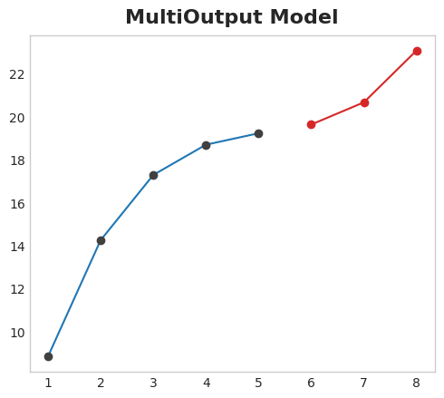
  • Use a model that produces multiple outputs naturally, with linear regression or neural networks, etc.
    
• Direct strategy
  • Train a separate model for each step in the horizon: one model forecasts 1-step ahead, another 2-steps ahead, and so on.
    
• Recursive strategy
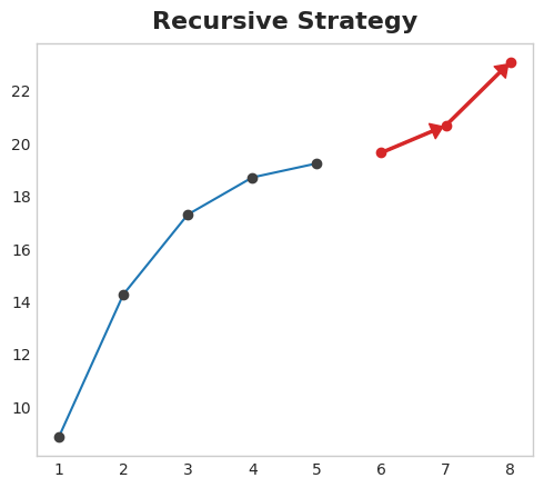
  • Train a single one-step model and use its forecasts to update the lag features for the next step.
    
• DirRec strategy
  • A combination of the direct and recursive strategies: train a model for each step and use forecasts from previous steps as new lag features.
    

Forecasting methods

We can choose methods depending on the time series patterns

• If the data exhibit stationarity properties
  • use mean and covariance will be enough
• If there is no trend nor seasonality
  • naive forecasting:
    • the future values of a time series will be equal to the last observed value
  • moving average:
    • sums up a series of time steps and the average will be the prediction for the next time step
• If there is trend and/or seasonality:
  • differencing (+moving average):
    • For example, if the seasonality period is 365 days, you will subtract the value at time t – 365 from the value at time t period and then use it to generate a moving average.
  • smoothing (on top of differencing and moving average)
    • to avoid noise in differencing data, you can smooth out past values before adding them back to the time differenced moving average. There are two ways to do this:
      • Trailing windows - This refers to getting the mean of past values to smooth out the value at the current time step. For example, getting the average of t=0 to t=6 to get the smoothed data point at t=6.
      • Centered windows - This refers to getting the mean of past and future values to smooth out the value at the current time step. For example, getting the average of t=0 to t=6 to get the smoothed data point at t=3.
    • exponential smoothing
      • forecasts are equal to a weighted average of past observations and the corresponding weights decrease exponentially as we go back in time
  • autoregression
  • ARIMA (autoregressive integrated moving average)
    • ARIMA models combine two approaches:
      • AutoRegressive model: forecasts correspond to a linear combination of past values of the variable.
      • Moving Average model: forecasts correspond to a linear combination of past forecast errors.
    • Both model require the time series to be stationary, differencing (Integrating) the time series may be a necessary step, i.e. considering the time series of the differences instead of the original one.
  • SARIMA (Seasonal ARIMA)
    • extends the ARIMA by adding a linear combination of seasonal past values and/or forecast errors.
  • Prophet:
    • a forecasting method developed by Facebook that uses a decomposable time series model with components for trend, seasonality, and holidays.
  • Long Short Term Memory

Partitioning in Time Series

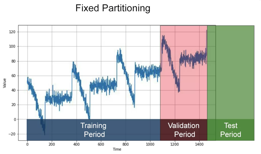
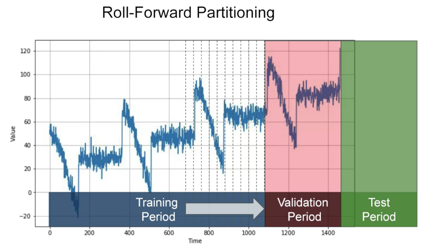
Roll-forward partitioning: start with a short training period, and we gradually increase it, say by one day at a time, or by one week at a time. At each iteration, we train the model on a training period. And we use it to forecast the following day, or the following week, in the validation period.